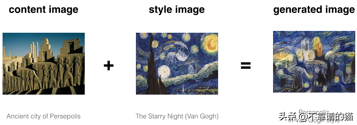
深度學(xué)習(xí)可以捕獲一個(gè)圖像的內(nèi)容并將其與另一個(gè)圖像的風(fēng)格相結(jié)合，這種技術(shù)稱為神經(jīng)風(fēng)格遷移。但是，神經(jīng)風(fēng)格遷移是如何運(yùn)作的呢？在這篇文章中，我們將研究神經(jīng)風(fēng)格遷移（NST）的基本機(jī)制。

神經(jīng)風(fēng)格遷移概述

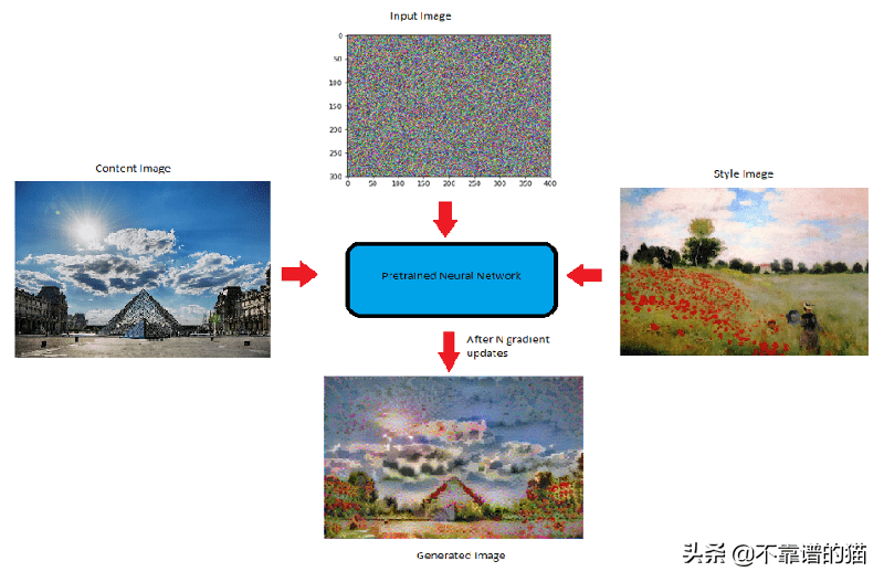
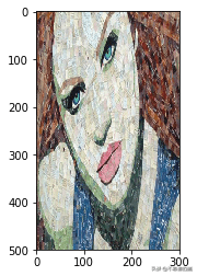
我們可以看到，生成的圖像具有內(nèi)容圖像的內(nèi)容和風(fēng)格圖像的風(fēng)格。可以看出，僅通過重疊圖像不能獲得上述結(jié)果。我們是如何確保生成的圖像具有內(nèi)容圖像的內(nèi)容和風(fēng)格圖像的風(fēng)格呢？

為了回答上述問題，讓我們來看看卷積神經(jīng)網(wǎng)絡(luò)（CNN）究竟在學(xué)習(xí)什么。

卷積神經(jīng)網(wǎng)絡(luò)捕獲到了什么

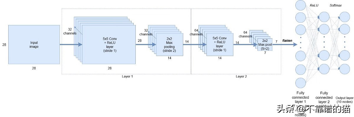
卷積神經(jīng)網(wǎng)絡(luò)的不同層

現(xiàn)在，在第1層使用32個(gè)filters ，網(wǎng)絡(luò)可以捕捉簡單的模式，比如直線或水平線，這對(duì)我們可能沒有意義，但對(duì)網(wǎng)絡(luò)非常重要，慢慢地，當(dāng)我們到第2層，它有64個(gè)filters ，網(wǎng)絡(luò)開始捕捉越來越復(fù)雜的特征，它可能是一張狗的臉或一輛車的輪子。這種捕獲不同的簡單特征和復(fù)雜特征稱為特征表示。

這里需要注意的是，卷積神經(jīng)網(wǎng)絡(luò)（CNN）并不知道圖像是什么，但他們學(xué)會(huì)了編碼特定圖像所代表的內(nèi)容。卷積神經(jīng)網(wǎng)絡(luò)的這種編碼特性可以幫助我們實(shí)現(xiàn)神經(jīng)風(fēng)格遷移。

卷積神經(jīng)網(wǎng)絡(luò)如何用于捕獲圖像的內(nèi)容和風(fēng)格

VGG19網(wǎng)絡(luò)用于神經(jīng)風(fēng)格遷移。VGG-19是一個(gè)卷積神經(jīng)網(wǎng)絡(luò)，可以對(duì)ImageNet數(shù)據(jù)集中的一百多萬個(gè)圖像進(jìn)行訓(xùn)練。該網(wǎng)絡(luò)深度為19層，并在數(shù)百萬張圖像上進(jìn)行了訓(xùn)練。因此，它能夠檢測(cè)圖像中的高級(jí)特征。

現(xiàn)在，CNN的這種“編碼性質(zhì)”是神經(jīng)風(fēng)格遷移的關(guān)鍵。首先，我們初始化一個(gè)噪聲圖像，它將成為我們的輸出圖像（G）。然后，我們計(jì)算該圖像與網(wǎng)絡(luò)中特定層（VGG網(wǎng)絡(luò)）的內(nèi)容和風(fēng)格圖像的相似程度。由于我們希望輸出圖像（G）應(yīng)該具有內(nèi)容圖像（C）的內(nèi)容和風(fēng)格圖像（S）的風(fēng)格，因此我們計(jì)算生成的圖像（G）的損失，即到相應(yīng)的內(nèi)容（C）和風(fēng)格（ S）圖像的損失。

有了上述直覺，讓我們將內(nèi)容損失和風(fēng)格損失定義為隨機(jī)生成的噪聲圖像。

NST模型

內(nèi)容損失

計(jì)算內(nèi)容損失意味著隨機(jī)生成的噪聲圖像(G)與內(nèi)容圖像(C)的相似性。為了計(jì)算內(nèi)容損失:

假設(shè)我們?cè)谝粋€(gè)預(yù)訓(xùn)練網(wǎng)絡(luò)(VGG網(wǎng)絡(luò))中選擇一個(gè)隱藏層(L)來計(jì)算損失。因此，設(shè)P和F為原始圖像和生成的圖像。其中，F(xiàn)[l]和P[l]分別為第l層圖像的特征表示。現(xiàn)在，內(nèi)容損失定義如下:

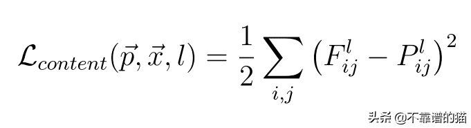
內(nèi)容成本函數(shù)

風(fēng)格損失

在計(jì)算風(fēng)格損失之前，讓我們看看“ 圖像風(fēng)格 ”的含義或我們?nèi)绾尾东@圖像風(fēng)格。

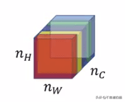
層l中的不同通道或特征映射

這張圖片顯示了特定選定層的不同通道或特征映射或filters。現(xiàn)在，為了捕捉圖像的風(fēng)格，我們將計(jì)算這些filters之間的“相關(guān)性”，也就是這些特征映射的相似性。但是相關(guān)性是什么意思呢?

讓我們借助一個(gè)例子來理解它：

上圖中的前兩個(gè)通道是紅色和黃色。假設(shè)紅色通道捕獲了一些簡單的特征(比如垂直線)，如果這兩個(gè)通道是相關(guān)的，那么當(dāng)圖像中有一條垂直線被紅色通道檢測(cè)到時(shí)，第二個(gè)通道就會(huì)產(chǎn)生黃色的效果。

現(xiàn)在，讓我們看看數(shù)學(xué)上是如何計(jì)算這些相關(guān)性的。

為了計(jì)算不同filters或信道之間的相關(guān)性，我們計(jì)算兩個(gè)filters激活向量之間的點(diǎn)積。由此獲得的矩陣稱為Gram矩陣。

但是我們?nèi)绾沃浪鼈兪欠裣嚓P(guān)呢?

如果兩個(gè)filters激活之間的點(diǎn)積大，則說兩個(gè)通道是相關(guān)的，如果它很小則是不相關(guān)的。以數(shù)學(xué)方式：

風(fēng)格圖像的Gram矩陣（S）：

這里k '和k '表示層l的不同filters或通道。我們將其稱為Gkk ' [l][S]。

用于風(fēng)格圖像的Gram矩陣

生成圖像的Gram矩陣（G）：

這里k和k'代表層L的不同filters或通道。讓我們稱之為Gkk'[l] [G]。

生成圖像的Gram矩陣

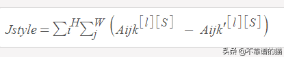
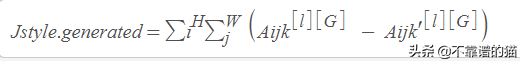
現(xiàn)在，我們可以定義風(fēng)格損失：

風(fēng)格與生成圖像的成本函數(shù)是風(fēng)格圖像的Gram矩陣與生成圖像的Gram矩陣之差的平方。

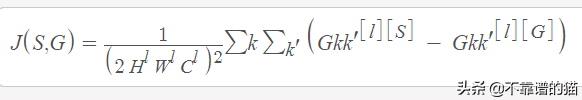
風(fēng)格成本函數(shù)

現(xiàn)在，讓我們定義神經(jīng)風(fēng)格遷移的總損失。

總損失函數(shù)：

總是內(nèi)容和風(fēng)格圖像的成本之和。在數(shù)學(xué)上，它可以表示為：

神經(jīng)風(fēng)格遷移的總損失函數(shù)

您可能已經(jīng)注意到上述等式中的Alpha和beta。它們分別用于衡量內(nèi)容成本和風(fēng)格成本。通常，它們?cè)谏傻妮敵鰣D像中定義每個(gè)成本的權(quán)重。

一旦計(jì)算出損失，就可以使用反向傳播使這種損失最小化，反向傳播又將我們隨機(jī)生成的圖像優(yōu)化為有意義的藝術(shù)品。

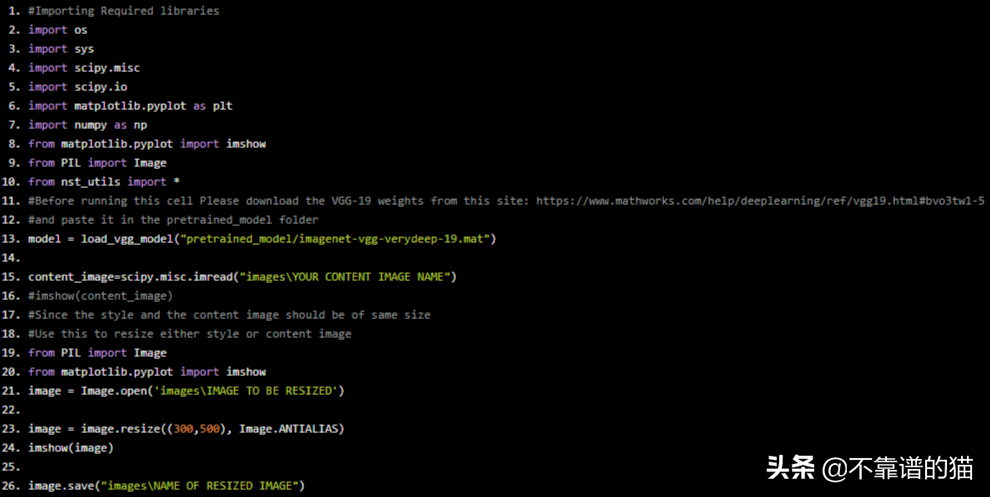
使用tensorflow實(shí)現(xiàn)神經(jīng)風(fēng)格遷移Python示例代碼：

#importing Required libraries
import os
import sys
import scipy.misc
import scipy.io
import matplotlib.pyplot as plt
import numpy as np
from matplotlib.pyplot import imshow
from PIL import Image
from nst_utils import *
#Before running this cell Please download the VGG-19 weights from this site: https://www.mathworks.com/help/deeplearning/ref/vgg19.html#bvo3tw1-5
#and paste it in the pretrained_model folder
model = load_vgg_model("pretrained_model/imagenet-vgg-verydeep-19.mat")
content_image=scipy.misc.imread("imagesYOUR ConTENT IMAGE NAME")
#imshow(content_image)
#Since the style and the content image should be of same size
#Use this to resize either style or content image
from PIL import Image
from matplotlib.pyplot import imshow
image = Image.open('imagesIMAGE TO BE RESIZED')
image = image.resize((300,500), Image.ANTIALIAS)
imshow(image)
image.save("imagesNAME OF RESIZED IMAGE")

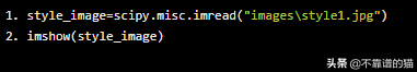
style_image=scipy.misc.imread("imagesstyle1.jpg")
imshow(style_image)

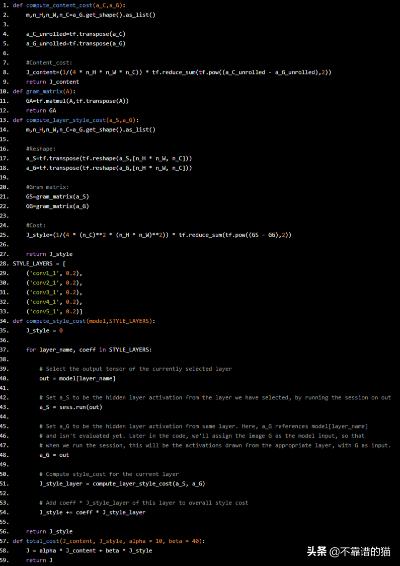
輔助函數(shù)

def compute_content_cost(a_C,a_G):
 m,n_H,n_W,n_C=a_G.get_shape().as_list()
 
 a_C_unrolled=tf.transpose(a_C)
 a_G_unrolled=tf.transpose(a_G)
 
 #Content_cost:
 J_content=(1/(4 * n_H * n_W * n_C)) * tf.reduce_sum(tf.pow((a_C_unrolled - a_G_unrolled),2))
 return J_content
def gram_matrix(A):
 GA=tf.matmul(A,tf.transpose(A))
 return GA
def compute_layer_style_cost(a_S,a_G):
 m,n_H,n_W,n_C=a_G.get_shape().as_list()
 
 #Reshape:
 a_S=tf.transpose(tf.reshape(a_S,[n_H * n_W, n_C]))
 a_G=tf.transpose(tf.reshape(a_G,[n_H * n_W, n_C]))
 
 #Gram matrix:
 GS=gram_matrix(a_S)
 GG=gram_matrix(a_G)
 
 #Cost:
 J_style=(1/(4 * (n_C)**2 * (n_H * n_W)**2)) * tf.reduce_sum(tf.pow((GS - GG),2))
 
 return J_style
STYLE_LAYERS = [
 ('conv1_1', 0.2),
 ('conv2_1', 0.2),
 ('conv3_1', 0.2),
 ('conv4_1', 0.2),
 ('conv5_1', 0.2)]
def compute_style_cost(model,STYLE_LAYERS):
 J_style = 0
 for layer_name, coeff in STYLE_LAYERS:
 # Select the output tensor of the currently selected layer
 out = model[layer_name]
 # Set a_S to be the hidden layer activation from the layer we have selected, by running the session on out
 a_S = sess.run(out)
 # Set a_G to be the hidden layer activation from same layer. Here, a_G references model[layer_name] 
 # and isn't evaluated yet. Later in the code, we'll assign the image G as the model input, so that
 # when we run the session, this will be the activations drawn from the appropriate layer, with G as input.
 a_G = out
 
 # Compute style_cost for the current layer
 J_style_layer = compute_layer_style_cost(a_S, a_G)
 # Add coeff * J_style_layer of this layer to overall style cost
 J_style += coeff * J_style_layer
 return J_style
def total_cost(J_content, J_style, alpha = 10, beta = 40):
 J = alpha * J_content + beta * J_style
 return J

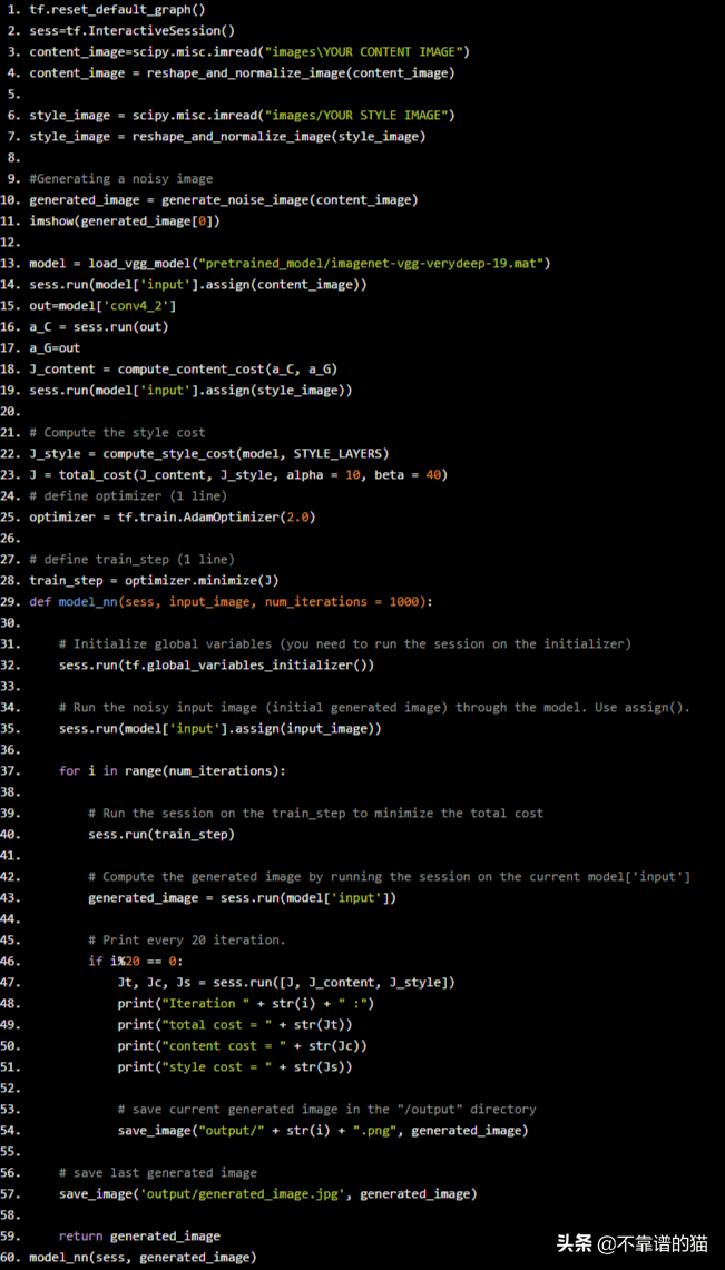
優(yōu)化及神經(jīng)網(wǎng)絡(luò)模型

tf.reset_default_graph()
sess=tf.InteractiveSession()
content_image=scipy.misc.imread("imagesYOUR ConTENT IMAGE")
content_image = reshape_and_normalize_image(content_image)
style_image = scipy.misc.imread("images/YOUR STYLE IMAGE")
style_image = reshape_and_normalize_image(style_image)
#Generating a noisy image
generated_image = generate_noise_image(content_image)
imshow(generated_image[0])
model = load_vgg_model("pretrained_model/imagenet-vgg-verydeep-19.mat")
sess.run(model['input'].assign(content_image))
out=model['conv4_2']
a_C = sess.run(out)
a_G=out
J_content = compute_content_cost(a_C, a_G)
sess.run(model['input'].assign(style_image))
# Compute the style cost
J_style = compute_style_cost(model, STYLE_LAYERS)
J = total_cost(J_content, J_style, alpha = 10, beta = 40)
# define optimizer (1 line)
optimizer = tf.train.AdamOptimizer(2.0)
# define train_step (1 line)
train_step = optimizer.minimize(J)
def model_nn(sess, input_image, num_iterations = 1000):
 
 # Initialize global variables (you need to run the session on the initializer)
 sess.run(tf.global_variables_initializer())
 
 # Run the noisy input image (initial generated image) through the model. Use assign().
 sess.run(model['input'].assign(input_image))
 
 for i in range(num_iterations):
 
 # Run the session on the train_step to minimize the total cost
 sess.run(train_step)
 
 # Compute the generated image by running the session on the current model['input']
 generated_image = sess.run(model['input'])
 # Print every 20 iteration.
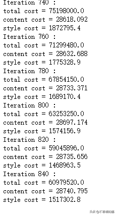
 if i%20 == 0:
 Jt, Jc, Js = sess.run([J, J_content, J_style])
 print("Iteration " + str(i) + " :")
 print("total cost = " + str(Jt))
 print("content cost = " + str(Jc))
 print("style cost = " + str(Js))
 
 # save current generated image in the "/output" directory
 save_image("output/" + str(i) + ".png", generated_image)
 
 # save last generated image
 save_image('output/generated_image.jpg', generated_image)
 
 return generated_image
model_nn(sess, generated_image)

最后

在這篇文章中，我們深入研究了神經(jīng)風(fēng)格遷移的工作原理。我們還討論了NST背后的數(shù)學(xué)。